ECE 5745 Section 3: ASIC Evaluation
- Author: Christopher Batten
- Date: February 14, 2020
Table of Contents
- Introduction
- Generating the Design
- Pushing the Design Through the Automated ASIC Flow
- Evaluating Cycle Time
- Evaluating Area
Introduction
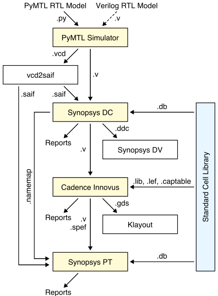
In this section, we will be using the automated ASIC toolflow to evaluate a fixed-latency and variable-latency iterative multiplier. As a reminder, here is the high-level view of the tools we will be using in the course. When using the automated ASIC toolflow there are many more steps, but this is still the high-level approach.
The first step is to start MobaXterm. From the Start menu, choose MobaXterm Educational Edition > MobaXterm Educational Edition. Then double click on ecelinux.ece.cornell.edu under Saved sessions in MobaXterm. Log in using your NetID and password. Click Yes when asked if you want to save your password. This will make it easier to open multiple terminals if you need to.
Once you are at the ecelinux prompt, source the setup script, clone
this repository from GitHub, and define an environment variable to keep
track of the top directory for the project.
% source setup-ece5745.sh
% mkdir $HOME/ece5745
% cd $HOME/ece5745
% git clone https://github.com/cornell-ece5745/ece5745-S03-asic-eval
% cd ece5745-S03-asic-eval
% TOPDIR=$PWD
Generating the Design
The first step is always to verify that our design works before we start
evaluating it. We should use the --test-verilog command line option to
ensure that the actual translated Verilog is functioning correctly.
% mkdir $TOPDIR/sim/build
% cd $TOPDIR/sim/build
% pytest ../lab1_imul/test
% pytest ../lab1_imul/test --test-verilog
The next step is to characterize the execution time in cycles both designs, and to also generate the corresponding Verilog RTL that we want to push through the flow.
% cd $TOPDIR/sim/build
% ../lab1_imul/imul-sim --impl rtl-fixed --input small --stats --dump-vcd --translate
% ../lab1_imul/imul-sim --impl rtl-var   --input small --stats --dump-vcd --translate
Make a note of the execution time in cycles and the average latency per multiply transaction for each design. Take a quick look at the generated Verilog.
% cd $TOPDIR/sim/build
% more lab1_imul_IntMulFixedLatRTL.v
% more lab1_imul_IntMulVarLatRTL.v
Pushing the Design Through the Automated ASIC Flow
We will start by pushing both the fixed-latency and variable-latency
multipliers completely through the flow, examine the final design, and
then we will start evaluating the cycle time, area, and energy. As we saw
last time, each design has a corresponding entry in the asic/designs
directory:
% cd $TOPDIR/asic/designs
% tree
% more IntMulFixedLatRTL/flow.py
% more IntMulVarLatRTL/flow.py
Inside the flow.py file, there are a lot of information, but the
important configuration is placed at the top of the file:
#-----------------------------------------------------------------------
# Parameters
#-----------------------------------------------------------------------

adk_name = 'freepdk-45nm'
adk_view = 'view-standard'

parameters = {
 'construct_path' : __file__,
 'design_name'    : 'lab1_imul_IntMulFixedLatRTL',
 'clock_period'   : 2.0,
 'adk'            : adk_name,
 'adk_view'       : adk_view,
 'topographical'  : True,
}
The adk_name specifies the targeted technology node and fabrication
process. The design_name is the name of the corresponding top-level
module. The clock_period is the target clock period we want to use for
synthesis and place-and-route.
To get started create a build directory and run the configure script. You need to explicitly specify which design you want to push through the flow when you run the configure script.
% cd $TOPDIR/asic
% mkdir build-fixed
% cd build-fixed
% ../configure --design ../designs/IntMulFixedLatRTL
% make list
The list Makefile target will display the various targets that you can
use to manage the flow. You can use the following to generate a figure of
the overall ASIC flow.
% cd $TOPDIR/asic/build-fixed
% make graph
You can open the generated graph.pdf file to see the figure. The
following two commands will perform synthesis (the front-end of the flow)
and then place-and-route (the back-end of the flow).
% cd $TOPDIR/asic/build-fixed
% make synopsys-dc-synthesis
% make cadence-innovus-place-route
% make summarize-results
It will take a few minutes to push the design through the flow. The automated flow takes longer than the manual steps we used before because the automated flow is using a much more sophisticated approach with many more optimization steps. Be aware that for larger designs it can take quite a while to push a design through the entire flow. Consider using just the ASIC flow front-end to ensure your design is synthesizable and to gain some rough early intuition on area and timing. Then you can iterate quickly and eventually focus on the ASIC flow back-end.
You should see some final summary results:
#=================================================================
# Post-Place-and-Route Results
#=================================================================

  vsrc       = lab1_imul_IntMulFixedLatRTL
  timestamp  = 2020-02-14 08:42
  area       = 895.622 # um^2
  constraint = 2.0 # ns
  slack      = 0.157 # ns
Our cycle time constraint was 2ns, and we have 0.157ns of positive slack. This means we “met timing”. If you end up with negative slack, then you need to rerun the tools with a longer target clock period until you can meet timing with no negative slack. The process of tuning a design to ensure it meets timing is called “timing closure”. In this course, we are primarily interested in design-space exploration as opposed to meeting some externally defined target timing specification. So you will need to sweep a range of target clock periods. Your goal is to choose the shortest possible clock period which still meets timing without any negative slack! This will result in a well-optimized design and help identify the “fundamental” performance of the design.
You can use the debug- targets to view the final design in Cadence
Innovus.
% make debug-cadence-innovus-place-route
You can use the design browser to help visualize how modules are mapped across the chip. Here are the steps:
- Choose Windows > Workspaces > Design Browser + Physical from the menu
- Hide all of the metal layers by pressing the number keys
- Browse the design hierarchy using the panel on the left
- Right click on a module, click Highlight, select a color
You can use the following steps in Cadence Innovus to display where the critical path is on the actual chip.
- Choose Timing > Debug Timing from the menu
- Right click on first path in the Path List
- Choose Highlight > Only This Path > Color
You can create a screen capture to create an amoeba plot of your chip using the Tools > Screen Capture > Write to GIF File. We recommend inverting the colors so your amoeba plot looks better in a report.
To Do On Your Own: Highlight the critical path and some of the key modules in the fixed-latency multiplier. Create an amoeba plot, copy it to the workstation, and open it using the default Windows viewer.
Evaluating Cycle Time
Our initial design has plenty of positive slack. Let’s now try pushing
the cycle time to see if we can produce a faster multiplier. Try pushing
the fixed-latency multiplier through the flow with a cycle time of 0.5ns
(i.e., 2GHz). To do this, you need to modify the clock_period in
flow.py, reconfigure the design, and rerun the flow.
% cd $TOPDIR/asic/build-fixed
% make clean-all
% ../configure --design ../designs/IntMulFixedLatRTL
% make info
% make synopsys-dc-synthesis
% make cadence-innovus-place-route
% make summarize-results
It is good to always good to start from a clean build and to use make
info first to ensure you are using the right design and clock
constraint. You can make a copy of the build directory if you want to
save your results from a previous push through the flow.
Now let’s see if we can explore the critical path in more detail. You can find a summary in the reports generated by Cadence Innovus.
% cd $TOPDIR/asic/build-fixed
% cat 6-cadence-innovus-place-route/reports/signoff.summary
This file will show you the worst-case negative slack (WNS) across many different path groups. You want to see which path group has the worst-case negative slack (i.e., the smallest value in the WNS row). In this case it is probably the Reg2Reg path group which includes all paths that start at a register and end at a register. Take a look the more detailed reports for just this path group.
% cd $TOPDIR/asic/build-fixed
% cat 6-cadence-innovus-place-route/reports/signoff_Reg2Reg.tarpt
The first path will be the worst-case path in that path group.
To Do On Your Own: Highlight the critical path on the datapath diagram for the fixed-latency multiplier. Annotate each component along the critical path with a rough estimate of its delay in picoseconds. Don’t forget to estimate the register clock-to-q delay and the register setup time. What components are consuming the most time along the critical path?
Let’s now try pushing the variable latency multiplier through the flow with the same clock constraint.
% mkdir $TOPDIR/asic/build-var
% cd $TOPDIR/asic/build-var
% ../configure --design ../designs/IntMulVarLatRTL
% make info
% make synopsys-dc-synthesis
% make cadence-innovus-place-route
% make summarize-results
You will see that the variable-latency multiplier cannot meet timing with
a 0.5ns clock period, so you will need to respin the design with a longer
clock period. Try using 0.5ns. Don’t forget to use make clean-all
before reconfiguring and to use make info to make sure you have things
setup correctly. Explore the critical path in more detail using the
reports from Cadence Innovus.
To Do On Your Own: Highlight the critical path on the datapath diagram for the variable-latency multiplier. Annotate each component along the critical path with a rough estimate of its delay in picoseconds. Don’t forget to estimate the register clock-to-q delay and the register setup time. What components are consuming the most time along the critical path?
Evaluating Area
Now that we have evaluated the cycle time, we can move on to evaluating the area. The post-place-and-route area report provides us the number of standard-cell instances and the area in square um for each component in our design.
% cd $TOPDIR/asic/build-fixed
% cat 6-cadence-innovus-place-route/reports/signoff.area.rpt

% cd $TOPDIR/asic/build-var
% cat 6-cadence-innovus-place-route/reports/signoff.area.rpt
To Do On Your Own: Highlight the critical path on the datapath diagram for the variable-latency multiplier. Annotate each component in the datapath diagram with a rough estimate of its area in square um. What components are consuming the most area? Compare the area between the fixed and variable latency multipliers. Where is the area overhead coming from?